Silkroads: Spreadsheet Balancing of Abundance

Key values are all in place. You can select trade routes – some of which will be more profitable than others. You can build infrastructure to make trading over long distances more feasible. Now what I need to do is ensure that abundance changes across the map – the rise and fall of selling-price for silk, spices, etc. – approaches a reasonable rate. This falloff needs to vary between somewhat profitable and very unprofitable: neighboring nodes with too high an abundance difference represent a dominant strategy, or an easy exploit which destroys the challenge of silkroads. If I can get rich trading between Babylon’s 1-abundance and neighboring Ur’s 0-abundance, what is the point of seeking out other search routes.

Many blog-posts ago, I explained my first pass at resource abundance distribution. Abundance – a value between 0 and 1 representing market saturation (0 sells high, 1 sells low) – can be seen for each resource in the bar-charts above. My first pass handled a few nodes strung across the silk road. Since then, I’ve added many more. All require more thorough treatment to create a balanced, challenging resource spread.

Managing these values by-eye and with trial-and-error would be possible, but extensive. When core values need to be quickly judged, designers employ a different tool.

Spreadsheeting

The task of showing numerous interdependent values – perhaps in the hundreds or thousands, allowing for tweaks, and with a customized display for easy reading, is perfectly handled by Microsoft’s spreadsheet software: Excel. I’ve been looking forward to using it to my advantage for the sake of predictive balancing.

To begin with, Excel can open my Goods.xml file directly:

From these values, I can determine a great deal. I’ll start with the abundance/valuePerKilo graph. A trade good’s value at any one node is given by the function:

localVPK = (-v + p) * a + v

Where v is the base valuePerKilo, p is prodCost, and a is local abundance (the x-axis). Writing this function into Excel’s cell function is easy enough, but I actually need it available in a lot of places. So, under the Developer tab, I can write it in Visual Basic as a custom function.

Public Function LocalVPK(vpk As Single, prodCost As Single, abundance As Single) As Single
LocalVPK = (-vpk + prodCost) * abundance + vpk
End Function

This was my first time using Visual Basic, but my experience with other programming makes these menial tasks easy to understand. This is just a custom mathematical function, which can give me the local value-per-kilo of any good, whenever I need it.

Making a table of possible values, between 0 and 1 abundance, I can graph the localVPK function for each good.

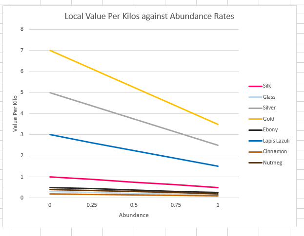
Again, this just demonstrates the value per kilo (v/kg) that a good would sell for at a node, for every possible abundance at that node. At 0 abundance, a good sells for its max price. At 1, it sells for its production cost.

Originally, the localVPK function I had in the game sold a good at 0 v/kg when at full abundance. This meant that at full abundance, a good would sell for nothing and could be purchased in infinite quantity for any amount of money, which didn’t make much mathematical or economic sense. The thinking behind this newer function is that, no matter how abundant a resource is, it will never be sold below its production cost, as the producer would be selling at an immediate loss. If it costs 1 value (1v) to mine 1kg of gold, selling that gold for 0.5v/kg is simply unthinkable.

Production cost – the lower limit of selling a good – is a fraction of maximum cost (base vpk). Currently, this is always 50%, but could easily be tweaked for more interesting market profiles.

Note that, despite this even ration, different resource graphs have different slopes: more valuable (per kg) resources, such as gold and silver, have steeper slopes. Less v/kg goods, such as glass and spices, have shallower profiles. This turns out to be very important.

Critical Delta-Abundance

The value I’m really interested in here is a complicated one. Assume I have a caravan travelling between two cities, 100km (1 Unity-unit) appart. Assume it can carry a maximum load of 20kg. Assume it’s trading silk, and that the first city has a higher abundance of silk than the second, so that it buys in cityA and sells in cityB. What is the minimum difference in abundance between cities A and B, needed to give the caravan enough profit to compensate for the cost of travelling.

This value is the Critical Delta-Abundance (CDA). It’s measured in difference in abundance per unit distance (da/100km). If the CDA is 0.3, and abundance at cityA = 1, while abundance at cityB = 0.7, the caravan can trade silk between the cities and make a net gain of exactly 0. If the difference in abundance between the two cities is less than the CDA, trading is not profitable. If it’s greater, trading is increasingly profitable.

Finding the CDA amounts to finding the delta-abundance from the delta-value (the value lost from travel expense), which is easily done with:

CDA = c / slope = c / (dx/dy)

where c is travel cost, and dx and dy are the differences in x and y. Since the graph is linear, dx and dy can be the entire width and height. Dividing the two yields the slope: 0 for flat, infinite for vertical, 1 for top-right diagonal.

The CDA should also take into account the quantity of goods being bought. This simply becomes:

c = q * (v – p)

q being quantity, v being base vpk, and p being production cost. This is important, because the slope of a graph for 1kg of silk is lower than the slope of a graph for 20kg silk.

Again, I’ve written this as a visual basic function:

Public Function CDA(distance As Single, amount As Single, vpkZero As Single, vpkOne As Single) As Single
CDA = (2 * distance) / (((vpkZero - vpkOne) * amount) / 1 - 0)
End Function

So now I can get the CDAs of each good, and at different distances.

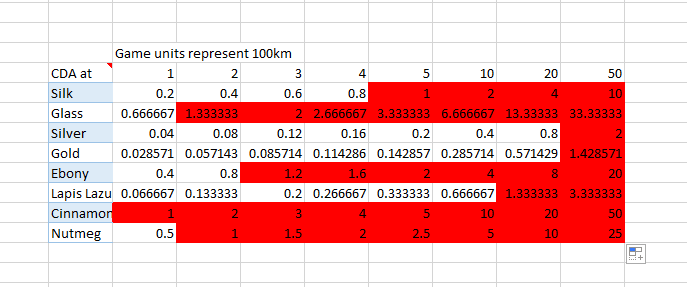
Remember: these values are the minimum delta-abundance at given distances needed for a profitable trade route of each resource. It also assumes no infrastructure – a mechanic which decreases the cost of travel. Where CDA is 1 or larger, trading is outright infeasible even at the most ideal situation (since abundance cannot differ by more than 1). So, for example, trading silk over a distance of anywhere above 500km simply cannot be profitable (without infrastructure upgrades). If the player was trading silk from China, and it took over 500km for the abundance to drop to 0 (which is only the distance between the entrance to China’s northern trading pass, and Kabul in Afghanistan, for example), then trading would be unprofitable.

An extreme case can be seen with Cinnamon. It requires a full drop in abundance over a distance of 100km – roughly the distance between central London and Oxford. With its current rate, it’s very difficult to trade.

The only resources worth trading over very long distances are the more valuable ones, with the steeper v/kg/a slopes. Gold, in particular, is still profitable across 2,000km, about the distance between London and St. Petersburg.

Looking at the abundance vs. price graph, it’s clear that the slope of the graph indicates how viable long-distance trading is. A steeper slope means the good can e traded further. As a result, I’ve tweaked the production costs of Gold, Silver, and Lapis, making them more expensive to produce, and thus a little less profitable.

There’s much more to be done. It’s time to apply these important values to the game.